PID controller - definition, operating principle, configuration and applications
Controller
PID controllers are used to influence specific meters. As smart 3-in-1-controllers, they prove themselves every day in numerous industrial systems and control very precisely to the setpoint. We provide you with the most important facts and figures about PID regulation.What is a PID-controller?
The compact controller can be adapted to a wide range of applications and is typically used as the PID controller. It works proportionally by integrating and differentiating (PID). Here the intensity of the individual components is adapted to the control process. This is done by measuring control parameters.
- Pb (proportional band),
- rt (reboot time) and
- dt (derivative time).
How do PID controllers work?
The operating principle of the PID controller is relatively simple to explain. Regardless of whether the controller is a temperature controller PID or a humidity controller PID, the controller always attempts to adjust a specific control variable to a set value based on the actual value. In this case, the P component amplifies the control deviation, the I component increases its output level in case of existing control deviation, and the D component counteracts the movement of the actual value. Components that are not required for management can be deactivated. Depending on the application, they are then controlled as PI controllers, P-controllers, PD controllers or I-controllers.
What applications are the PID controllers used in?
The PID structure exhibits the best control response for most applications. As a result, compact controllers PID are very common in the field of temperature control. They also allow direct connection of temperature sensors RTD and thermocouples. Some controlled variables require certain components to be turned off, including speed and flow.
What is the meaning behind the components PID and the corresponding control parameters?
The P - component Reacts very quickly and enhances differential control; his constant control deviation has an adverse effect. The responsible control parameter is the Pb proportional band. With a smaller Pb dimension, the controller becomes faster and the control deviation is smaller. However, the overall system tends to fluctuate more and more.
The Component Eliminates control deviation. If the reset time rt is set shorter, the controller ramps up its output level faster and also resists control drift faster. However, if the setting is too small, oscillatory behavior will also occur.
The D component This means to the heating controller that the component decreases when the actual value increases, and increases when the actual value decreases. The described behavior has a damping effect. The critical parameter is the derivative time dt. The larger dt is set, the greater the described effect.
Purchase of PID controllers
How to optimize PID controllers?
The behavior of the control process always depends on the operating point. Therefore, before tuning, the plant must be set to an operating state for which favorable control parameters are later expected. For example, a furnace must be loaded before tuning, or a demand for a flow heater must be generated. If a target value must be specified during tuning, this must be within the subsequent operating range.
If comparable installations/control loops exist, the control parameters used in them may be used on a trial basis. If this approach does not achieve the goal, one of the following optimization methods can be used.
Oscillation method according to Ziegler and Nichols
This method is used for relatively fast managed systems. For preparation, the P structure is parameterized and the Pb value is set to a relatively large value. The following figure determines the set point value that lies within the subsequent operating range.
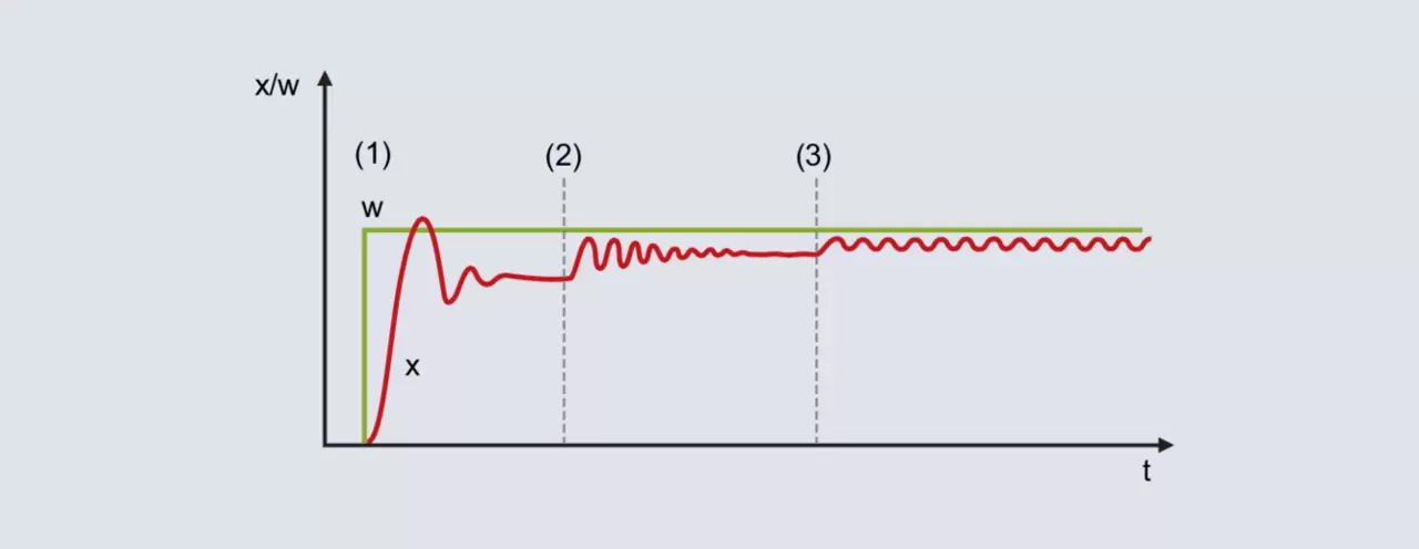
With a relatively large proportional band, the actual value moves towards the final value with a slight tendency to fluctuate [Figure 52 (1)]. Due to the non-existent I structure, there is a constant control deviation.
Pb decreases (Figure 52 [2]): The actual value increases and moves towards the final value with a greater tendency to fluctuate. Under certain circumstances, the proportional band is reduced by several times until the actual value fluctuates continuously (Figure 52 [3]). The proportional band required for this behavior is called Pbc (Pb critical) and should be determined as accurately as possible (do not reduce Pb in excessively large steps).
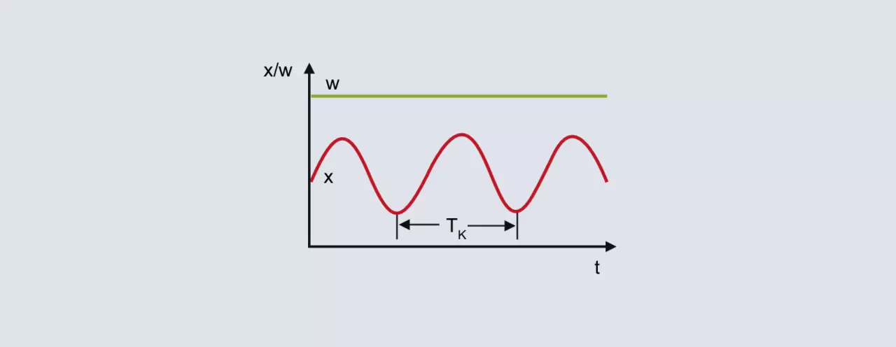
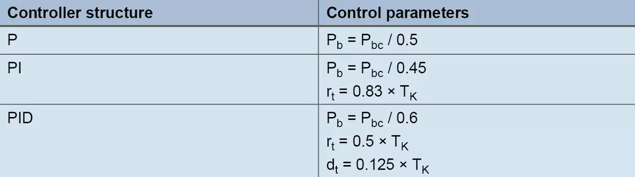
From the continuous fluctuation of the actual value in the upper figure, the critical period duration Tc represents the second characterizing parameter that must be determined for the method. The critical period duration Tc (in seconds) is calculated from the time interval between 2 minimum values, e.g. To determine the control parameters, Pbc and Tc are inserted into the following table for the intended controller structure:
Method based on the reaction stage of the process according to Chin, Chron and Reswick
With this method, control parameters are calculated relatively quickly, even for slow control processes. The method is applied to both second-order processes and is characterized by the fact that it distinguishes between formulas for transient behavior and disturbance behavior. For empirical rules based on the step, the transfer coefficient of the control process, the delay time and the compensation time are calculated.
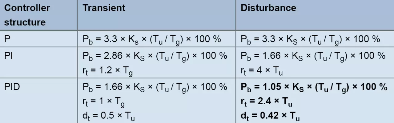
Example:
The controller with structure PID should be used for laboratory furnace. The goal is to achieve good disturbance behavior, and typical set point values are 200 °C. The output level is gradually increased in manual mode until the actual value is slightly lower than the future set value (wait for the corresponding compensation processes). For example, a temperature of 180 °C is achieved with an output level of 60 %. Starting from 60 %, the output level suddenly increases to 80 % and the actual value is recorded.
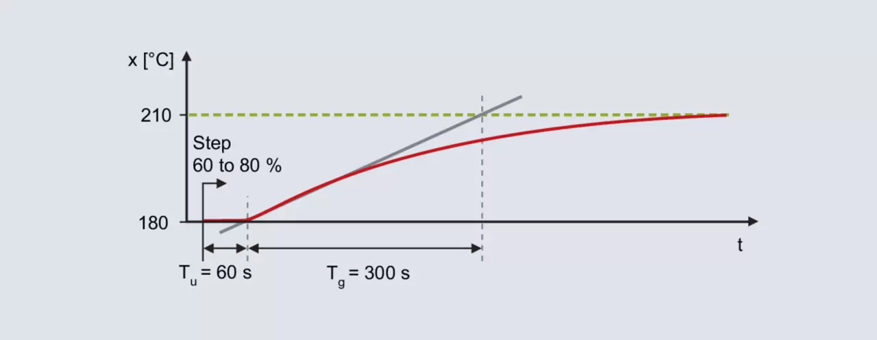
The reaction to the step is determined using the inflection tangent: delay time Тu = 60 s, compensation time Тг = 300 s. The control process gain is the result of the change in actual value divided by the output step.

Using rules of thumb, this leads to the following disturbance behavior parameters:



The output step must be performed in the area of the subsequent operating point. Additionally, the step size must be set high enough to allow analysis of the progress of the actual value. Once the output stage has been specified, it is necessary to wait for the final value of the actual value. An alternative to saving time is the method according to the rate of rise.
Method according to growth rate
Regarding the step change specification, the procedure is the same as for the process step response based method. Before changing the step, an output level is specified that results in an actual value that is slightly less than the specified value used later.
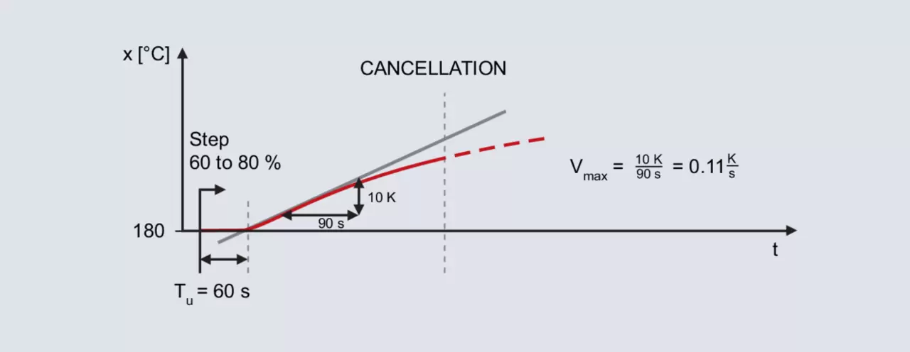
The pitch change is again specified for the already mentioned laboratory furnace, with the subsequent operating point also being 200 °C. Specifying the output level 60 % in manual mode results in the actual value 180 °C. The output level suddenly increases to 80 %.
After specifying a step change, the actual value increases after a while. Recording continues until the actual value reaches its maximum slope. The inflection tangent and the delay time determined by this method are also drawn. The second characterizing parameter is the maximum ascent speed, which corresponds to the inflection tangent. The maximum rate of ascent can be determined by plotting the slope triangle on the inflector tangent:

The calculated values of Vmax (0,11 K/s) and Tu (60 s) are used in the following formulas:
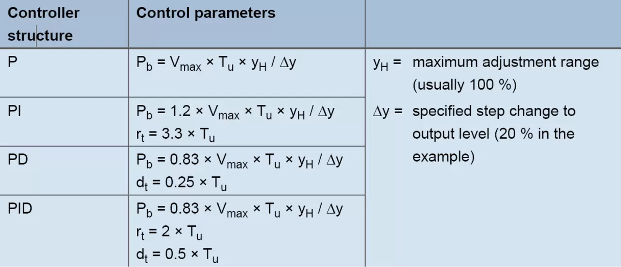
For controller PID with formulas the following values arise:



Empirical method for calculating control parameters
This method is used to sequentially calculate the optimal settings for components P, D and I. Starting from the initial state (output level 0 %), a typical setpoint value is specified each time; therefore, the method is only suitable for relatively fast control processes (such as fast temperature control processes or control variables such as speed or flow).
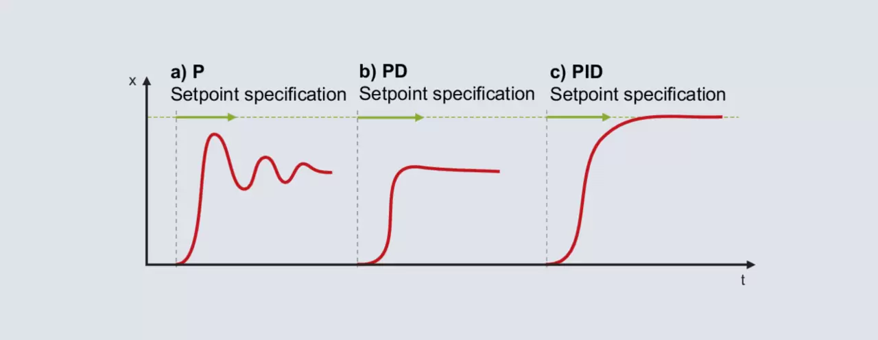
The P structure is activated for the controller. The proportional band is set relatively large (the size depends on the control process) and the set point value is set in the subsequent operating range. The actual value will move slowly towards the final value and a relatively large control deviation will be produced. The set point is then set with an increasingly smaller proportional band Pb. The goal is to achieve Pb, with which the actual value reaches its stable final value after 2-3 complete oscillations (Figure 56a). For a smooth start, the structure must be switched from P to PD. Starting with a small adjustment for the derivative time, the set point is specified with increasingly larger dt. If the actual value reaches its final value with as little fluctuation as possible, dt is in the optimal position (Figure 56b).
NoteOnce the controller sets the output level to 0% even once during startup, it means dt is set too large.
Component I is activated when the structure switches to PID. The optimal reset time rt is usually set to 4 times the previously determined dt. Figure 56c shows the response for setting rt = 4 × dt.
On some processes it is not possible to activate all components. If the P-structure already produces an unregulated response with a large Pb, then using the P- or D-structure will not work. Controller I should be used instead.
If controller P has been successfully configured, but the introduction of component D makes the control loop unstable, structure PI is used.
How can I reoptimize the PID controller manually?
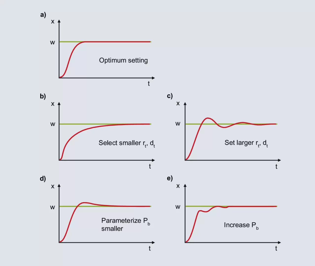
Using one of the tuning methods outlined in this chapter will likely result in a stable, but not optimal, control response. The control result can be further improved by manual adjustment. If the controller response PID can be mapped to one of the curves 62b - 62e, you will find information here for further configuration.
a)
The diagram shows the optimal behavior for the PID controller.
b)
After specifying the set point value, the actual value increases sharply until it reaches the proportional band. If the actual value falls within the proportional band, the P component is reduced and the I component adjusts the value to the set point value. The increase in the I component occurs slowly due to the relatively large rt and the control deviation is slowly eliminated. For faster integration, rt should be set smaller; dt also decreases according to the relation dt/rt = 1/4.
c)
When the actual value enters the proportional band, the I component increases the output level. The increase continues until the actual value reaches the set point value. In the example shown, component I produces an excess output level until the control drift is eliminated and the actual value exceeds the set point value. If there is a negative control deviation, the output level decreases too quickly and the actual value falls below the setpoint, etc. A symmetrical oscillation of the actual value around the setpoint indicates that rt is too small. rt must be increased and dt must also be increased according to the ratio dt/rt = 1/4.
d)
Component I is formed from the moment the actual value enters the proportional band until the control deviation is eliminated. Due to the large Pb, component I already begins to form its output level at a large control deviation. Due to the large control deviation at the beginning, component I builds its output level relatively quickly. When the control deviation is eliminated, the I component is too large and the actual value exceeds the target value. At a smaller setting for Pb, if there are smaller control deviations, component I begins to build up its output level at a corresponding slower rate. The one-time excess depicted becomes more incredible.
e)
With Pb set too low, the output level of the P component drops shortly before reaching the set value. When the actual value enters the proportional band, the P component decreases sharply and the actual value decreases. Due to larger control deviation, the output level becomes larger and the actual value increases. In proportional band, small changes in the actual value lead to large changes in the output level, resulting in a high tendency to oscillate. This is calmed down by increasing the proportional band.
Our services for you